Tutorial
Introduction
This tutorial will walk you through the creation and simulation of a PySB model.
First steps
Once you have installed PySB, run the following commands from a Python interpreter to check that the basic functionality is working. This will define a model that synthesizes a molecule “A” at the rate of 3 copies per second, simulates that model from t=0 to 60 seconds and displays the amount of A sampled at intervals of 10 seconds:
>>> from pysb import *
>>> from pysb.integrate import Solver
>>> Model()
<Model '<interactive>' (monomers: 0, rules: 0, parameters: 0, compartments: 0) at ...>
>>> Monomer('A')
Monomer('A')
>>> Parameter('k', 3.0)
Parameter('k', 3.0)
>>> Rule('synthesize_A', None >> A(), k)
Rule('synthesize_A', None >> A(), k)
>>> t = [0, 10, 20, 30, 40, 50, 60]
>>> solver = Solver(model, t)
>>> solver.run()
>>> print(solver.y[:, 0])
[   0.   30.   60.   90.  120.  150.  180.]
Creating a model
The example above notwithstanding, PySB model definition is not meant to be
performed in an interactive environment. The proper way to create a model is to
write the code in a .py file which can then be loaded interactively or in other
scripts for analysis and simulation. Here are the Python statements necessary to
define the model from First steps above. Save this code in a file named
tutorial_a.py (you can find a copy of this file and all other named scripts
from the tutorial in pysb/examples/):
from pysb import *

Model()
Monomer('A')
Parameter('k', 3.0)
Rule('synthesize_A', None >> A(), k)
Note that we did not import pysb.integrate, define the t variable or
create a Solver object. These are part of model usage, not definition, so
they do not belong here.
You may also be wondering why there are no assignment statements to be found.
This is because every PySB model component automatically assigns itself to a
variable named identically to the component’s name (A, k and
synthesize_A above), or model in the case of the Model object
itself. This is not standard Python behavior but it makes models much more
readable. The Component section below explains a bit more about this feature,
and technical readers can find even more in the Self-export section.
Using a model
Now that we have created a model file, we will see how to load it and do
something with it. Here is run_tutorial_a.py, the code corresponding to the
rest of the example from First steps.
from __future__ import print_function
from pysb.simulator import ScipyOdeSimulator
from tutorial_a import model

if __name__ == '__main__':
    t = [0, 10, 20, 30, 40, 50, 60]
    simulator = ScipyOdeSimulator(model, tspan=t)
    simresult = simulator.run()
    print(simresult.species)
The one line that’s been added relative to the original listing is from
tutorial_a import model. Since PySB models are just Python code, we use the
standard python import mechanism to load them. The variable model which
holds the Model object is explicitly chosen for import. All other model
components defined in tutorial_a.py are accessible through model, so
there is little need to import them separately.
Model creation in depth
Every model file must begin with these two lines:
from pysb import *
Model()
The first line brings in all of the Python classes needed to define a model. The
second line creates an instance of the Model class and implicitly assigns
this object to the variable model. We won’t have to refer to model
within the model file itself, rather this is the symbol we will later import
from other code in order to make use of the model.
The rest of the model file will be component declarations. There are several
types of components, some required and others optional. The required types are
Monomer, Parameter and Rule – we have already encountered these in
tutorial_a.py. The optional ones are Observable and Compartment.
Each of these component types is represented by a Python class which inherits
from the base class Component. The following sections will explain what each
of these component types does in a model and how to create them.
Component
The base Component class is never explicitly used in a model, but it defines
two pieces of basic functionality that are common to all component types. The
first is a name attribute, which is specified as the first argument to the
constructor for all subclasses of Component. The second is the “self-export”
functionality, which automatically assigns every component to a local variable
named for its name attribute. Self-export helps streamline model definition,
making it feel much more like a domain-specific language like BNGL or Kappa. A
justification for the technically-minded for this somewhat unusual behavior may
be found in the Self-export section near the end of the tutorial.
Monomer
Monomers are the indivisible elements that will make up the molecules and
complexes whose behavior you intend to model. Typically they will represent a
specific protein or other biomolecule such as “EGFR” or “ATP”. Monomers have a
name (like all components) as well as a list of sites. Sites are named
locations on the monomer which can bind with a site on another monomer and/or
take on a state. Binding merely represents aggregation, not necessarily a
formal chemical bond. States can range from the biochemically specific (e.g.
“phosphorylated/unphosphorylated” to the generic (e.g. “active/inactive”). The
site list is technically optional (as seen in tutorial_a.py) but only the
simplest toy models will be able to get by without them.
The Monomer constructor takes a name, followed
by a list of site names, and finally a dict specifying the allowable states for
the sites. Sites used only for binding may be omitted from the dict.
Here we will define a monomer representing the protein Raf, for use in a model of the MAPK signaling cascade. We choose to give our Raf monomer two sites: s represents the serine residue on which it is phosphorylated by Ras to activate its own kinase activity, and k represents the catalytic kinase domain with which it can subsequently phosphorylate MEK. Site s can take on two states: ‘u’ for unphosphorylated and ‘p’ for phosphorylated:
Monomer('Raf', ['s', 'k'], {'s': ['u', 'p']})
Now let’s provide a definition for MEK, the substrate of Raf. MEK has two serine residues at positions 218 and 222 in the amino acid sequence which are both phosphorylated by Raf. We can’t call them both s as site names must be unique within a monomer, so we’ve used the residue numbers in the sites’ names to distinguish them: s218 and s222. MEK has a kinase domain of its own for which we’ve again used k:
Monomer('MEK', ['s218', 's222', 'k'], {'s218': ['u', 'p'], 's222': ['u', 'p']})
Adding these two monomer definitions to a new model file tutorial_b.py
yields the following:
from pysb import *

Model()
Monomer('Raf', ['s', 'k'], {'s': ['u', 'p']})
Monomer('MEK', ['s218', 's222', 'k'], {'s218': ['u', 'p'], 's222': ['u', 'p']})
We can import this model in an interactive Python session and explore its monomers:
>>> from tutorial_b import model
>>> model.monomers
ComponentSet([
 Monomer('Raf', ['s', 'k'], {'s': ['u', 'p']}),
 Monomer('MEK', ['s218', 's222', 'k'], {'s218': ['u', 'p'], 's222': ['u', 'p']}),
 ])
>>> [m.name for m in model.monomers]
['Raf', 'MEK']
>>> model.monomers[0]
Monomer('Raf', ['s', 'k'], {'s': ['u', 'p']})
>>> model.monomers.keys()
['Raf', 'MEK']
>>> model.monomers['MEK']
Monomer('MEK', ['s218', 's222', 'k'], {'s218': ['u', 'p'], 's222': ['u', 'p']})
>>> model.monomers['MEK'].sites
['s218', 's222', 'k']
The Model class has a container for each component type, for example
monomers holds the monomers. These component objects are the very same ones
you defined in your model script – they were implicitly added to the model’s
monomers container by the self-export system. This container is a
ComponentSet, a special PySB class which acts like a list, a dict and a set
rolled into one, although it can only hold Component objects and can only be
appended to (never deleted from). Its list personality allows you to iterate
over the components or index an individual component by integer position, with
the ordering of the values corresponding to the order in which the components
were defined in the model. Its dict personality allows you to index an
individual component with its string name and use the standard keys and
items methods. The set personality allows set operations with ordering
retained. For binary set operators, the left-hand operand’s ordering takes
precedence.
We can also access the fields of a Monomer object such as name and
sites. See the PySB core (pysb.core) section of the module reference for
documentation on the fields and methods of all the component classes.
Parameter
Parameters are constant numerical values that represent biological constants. A parameter can be used as a reaction rate constant, compartment volume or initial (boundary) condition for a molecular species. Other than name, the only other attribute of a parameter is its numerical value.
The Parameter constructor takes the name and
value as its two arguments. The value is optional and defaults to 0.
Here we will define three parameters: a forward reaction rate for the binding of Raf and MEK and initial conditions for those two proteins:
Parameter('kf', 1e-5)
Parameter('Raf_0', 7e4)
Parameter('MEK_0', 3e6)
Add these parameter definitions to our tutorial_b model file
to create tutorial_c.py:
from pysb import *

Model()
Monomer('Raf', ['s', 'k'], {'s': ['u', 'p']})
Monomer('MEK', ['s218', 's222', 'k'], {'s218': ['u', 'p'], 's222': ['u', 'p']})
Parameter('kf', 1e-5)
Parameter('Raf_0', 7e4)
Parameter('MEK_0', 3e6)
Then explore the parameters container:
>>> from tutorial_c import model
>>> model.parameters
ComponentSet([
 Parameter('kf', 1e-05),
 Parameter('Raf_0', 70000.0),
 Parameter('MEK_0', 3000000.0),
 ])
>>> model.parameters['Raf_0'].value
70000.0
Parameters as defined are unitless, so you’ll need to maintain unit consistency
on your own. Best practice is to use number of molecules for species
concentrations (i.e. initial conditions) and S.I. units for everything else:
unimolecular rate constants in  , bimolecular rate constants in
 , compartment volumes in
  , etc.
In the following sections we will see how parameters are used to build other model components.
Rules
Rules define chemical reactions between molecules and complexes. A rule consists of a name, a pattern describing which molecular species should act as the reactants, another pattern describing how reactants should be transformed into products, and parameters denoting the rate constants.
The Rule constructor takes a name, a
RuleExpression containing the reactant and product patterns (more on that
below) and one or two Parameter objects for the rate constants. It also
takes several optional boolean flags as kwargs which alter the behavior of the
rule in certain ways.
Rules, as described in this section, comprise the basic elements of procedural instructions that encode biochemical interactions. In its simplest form a rule is a chemical reaction that can be made general to a range of monomer states or very specific to only one kind of monomer in one kind of state. We follow the style for writing rules as described in BioNetGen but the style proposed by Kappa is quite similar with only some differences related to the implementation details (e.g. mass-action vs. stochastic simulations, compartments or no compartments, etc). We will write two rules to represent the interaction between the reactants and the products in a two-step manner.
The general pattern for a rule consists of the statement Rule and in parenthesis a series of statements separated by commas, namely the rule name (string), the rule interactions, and the rule parameters. The rule interactions make use of the following operators:
*+* operator to represent complexation
*|* operator to represent backward/forward reaction
*>>* operator to represent forward-only reaction
*%* operator to represent a binding interaction between two species
Note
PySB used to use the <> operator for reversible rules, but that operator was removed in Python 3. All new models should use the | operator instead. Support for the <> in PySB with Python 2 will be removed in a future version of PySB.
To illustrate the use of the operators and the rule syntax we write the complex formation reaction with labels illustrating the parts of the rule:
Rule('C8_Bid_bind', C8(b=None) + Bid(b=None, S='u') | C8(b=1) % Bid(b=1, S='u'), *[kf, kr])
          |              |     |           |        |     |    |     |             |
          |              |     |           |        |     |    |     |            parameter list
          |              |     |           |        |     |    |     |
          |              |     |           |        |     |    |    bound species
          |              |     |           |        |     |    |
          |              |     |           |        |     |   binding operator
          |              |     |           |        |     |
          |              |     |           |        |    bound species
          |              |     |           |        |
          |              |     |           |        forward/backward operator
          |              |     |           |
          |              |     |          unbound species
          |              |     |
          |              |    complexation / addition operator
          |              |
          |             unbound species
         rule name
The rule name can be any string and should be enclosed in single (‘) or double (”) quotation marks. The species are instances of the monomers in a specific state. In this case we are requiring that C8 and Bid are both unbound, as we would not want any binding to occur with species that are previously bound. The complexation or addition operator tells the program that the two species are being added, that is, undergoing a transition, to form a new species as specified on the right side of the rule. The forward/backward operator states that the reaction is reversible. Finally the binding operator indicates that there is a bond formed between two or more species. This is indicated by the matching integer (in this case 1) in the bonding site of both species along with the binding operator. If a non-reversible rule is desired, then the forward-only operator can be replaced for the forward/backward operator.
In order to actually change the state of the Bid protein we must now edit the monomer so that have an actual state site as follows:
Monomer('Bid', ['b', 'S'], {'S':['u', 't']})
Having added the state site we can now further specify the state of the Bid protein when it undergoes rule-based interactions and explicitly indicate the changes of the protein state.
With this state site added, we can now go ahead and write the rules that will account for the binding step and the unbinding step as follows:
Rule('C8_Bid_bind', C8(b=None) + Bid(b=None, S='u') | C8(b=1) % Bid(b=1, S='u'), kf, kr)
Rule('tBid_from_C8Bid', C8(b=1) % Bid(b=1, S='u') >> C8(b=None) + Bid(b=None, S='t'), kc)
As shown, the initial reactants, C8 and Bid initially in the
unbound state and, for Bid, in the ‘u’ state, undergo a complexation
reaction and further a dissociation reaction to return the original
C8 protein and the Bid protein but now in the ‘t’ state,
indicating its truncation. Make these additions to your
mymodel.py file. After you are done, your file should look
like this:
# import the pysb module and all its methods and functions
from pysb import *

# instantiate a model
Model()

# declare monomers
Monomer('C8', ['b'])
Monomer('Bid', ['b', 'S'], {'S': ['u', 't']})

# input the parameter values
Parameter('kf', 1.0e-07)
Parameter('kr', 1.0e-03)
Parameter('kc', 1.0)

# now input the rules
Rule('C8_Bid_bind', C8(b=None) + Bid(b=None, S='u') | C8(b=1) % Bid(b=1, S='u'), kf, kr)
Rule('tBid_from_C8Bid', C8(b=1) % Bid(b=1, S='u') >> C8(b=None) + Bid(b=None, S='t'), kc)
Once you are done editing your file, start your ipython (or
python) interpreter and type the commands at the prompts below. Once
you load your model you should be able to probe and check that you
have the correct monomers, parameters, and rules. Your output should
be very similar to the one presented (output shown below the '>>>'
python prompts).:
>>> import mymodel as m
>>> m.model.monomers
   ComponentSet([
    Monomer('C8', ['b']),
    Monomer('Bid', ['b', 'S'], {'S': ['u', 't']}),
    ])
>>> model.parameters
   ComponentSet([
    Parameter('kf', 1e-07),
    Parameter('kr', 0.001),
    Parameter('kc', 1.0),
    Parameter('C8_0', 1000.0),
    Parameter('Bid_0', 10000.0),
    ])
>>> m.model.rules
   ComponentSet([
    Rule('C8_Bid_bind', C8(b=None) + Bid(b=None, S='u') | C8(b=1) % Bid(b=1, S='u'), kf, kr),
    Rule('tBid_from_C8Bid', C8(b=1) % Bid(b=1, S='u') >> C8(b=None) + Bid(b=None, S='t'), kc),
    ])
With this we are almost ready to run a simulation; all we need now is to specify the initial conditions of the system.
Observables
In our model we have two initial species (C8 and Bid) and one
output species (tBid). As can be seen in the ODEs derived from the
reactions above, there are four mathematical species needed to
describe the evolution of the system (i.e. C8, Bid, tBid, and
C8:Bid). Although this system is rather small, there are situations
when we will have many more species than we care to monitor or
characterize throughout the time evolution of the ODEs. In
addition, it will often happen that the desirable species are
combinations or sums of many other species. For this reason the
rules-based engines we currently employ implement the Observables
call which automatically collects the necessary information and
returns the desired species. In our case, we will monitor the amount
of free C8, unbound Bid, and active tBid. To specify the
observables enter the following lines in your mymodel.py file
as follows:
Observable('obsC8', C8(b=None))
Observable('obsBid', Bid(b=None, S='u'))
Observable('obstBid', Bid(b=None, S='t'))
As shown, the observable can be a species. As we will show later the observable can also contain wild-cards and given the “don’t care don’t write” approach to rule-writing, it can be a very powerful approach to observe activated complexes.
Initial conditions
Having specified the monomers, the parameters and the rules we
have the basics of what is needed to generate a set of ODEs and run a
model. From a mathematical perspective a system of ODEs can only be
solved if a bound is placed on the ODEs for integration. In our case,
these bounds are the initial conditions of the system that indicate
how much non-zero initial species are present at time t=0s in the
system. In our system, we only have two initial species, namely C8
and Bid so we need to specify their initial concentrations. To do
this we enter the following lines of code into the mymodel.py
file:
Parameter('C8_0', 1000)
Parameter('Bid_0', 10000)
Initial(C8(b=None), C8_0)
Initial(Bid(b=None, S='u'), Bid_0)
A parameter object must be declared to specify the initial condition rather than just giving a value as shown above. Once the parameter object is declared (i.e. C8_0 and Bid_0) it can be fed to the Initial definition. Now that we have specified the initial conditions we are basically ready to run simulations. We will add an observables call in the next section prior to running the simulation.
Simulation and analysis
By now your mymodel.py file should look something like this:
# import the pysb module and all its methods and functions
from pysb import *

# instantiate a model
Model()

# declare monomers
Monomer('C8', ['b'])
Monomer('Bid', ['b', 'S'], {'S':['u', 't']})

# input the parameter values
Parameter('kf', 1.0e-07)
Parameter('kr', 1.0e-03)
Parameter('kc', 1.0)

# now input the rules
Rule('C8_Bid_bind', C8(b=None) + Bid(b=None, S='u') | C8(b=1) % Bid(b=1, S='u'), *[kf, kr])
Rule('tBid_from_C8Bid', C8(b=1) % Bid(b=1, S='u') >> C8(b=None) + Bid(b=None, S='t'), kc)

# initial conditions
Parameter('C8_0', 1000)
Parameter('Bid_0', 10000)
Initial(C8(b=None), C8_0)
Initial(Bid(b=None, S='u'), Bid_0)

# Observables
Observable('obsC8', C8(b=None))
Observable('obsBid', Bid(b=None, S='u'))
Observable('obstBid', Bid(b=None, S='t'))
You can use a few commands to check that your model is defined
properly. Start your ipython (or python) interpreter and enter the
commands as shown below. Notice the output should be similar to the
one shown (output shown below the '>>>'` prompts):
>>> import mymodel as m
>>> m.model.monomers
   ComponentSet([
    Monomer('C8', ['b']),
    Monomer('Bid', ['b', 'S'], {'S': ['u', 't']}),
    ])
>>> m.model.parameters
   ComponentSet([
    Parameter('kf', 1e-07),
    Parameter('kr', 0.001),
    Parameter('kc', 1.0),
    Parameter('C8_0', 1000.0),
    Parameter('Bid_0', 10000.0),
    ])
>>> m.model.observables
   ComponentSet([
    Observable('obsC8', C8(b=None)),
    Observable('obsBid', Bid(b=None, S='u')),
    Observable('obstBid', Bid(b=None, S='t')),
    ])
>>> m.model.initials
   [Initial(C8(b=None), C8_0), Initial(Bid(b=None, S='u'), Bid_0)]
>>> m.model.rules
   ComponentSet([
    Rule('C8_Bid_bind', C8(b=None) + Bid(b=None, S='u') | C8(b=1) % Bid(b=1, S='u'), kf, kr),
    Rule('tBid_from_C8Bid', C8(b=1) % Bid(b=1, S='u') >> C8(b=None) + Bid(b=None, S='t'), kc),
    ])
With this we are now ready to run a simulation! The parameter values for the simulation were taken directly from typical values in the paper about extrinsic apoptosis signaling. To run the simulation we must use a numerical integrator. Common examples include LSODA, VODE, CVODE, Matlab’s ode15s, etc. We will use two python modules that are very useful for numerical manipulation. We have adapted the integrators in the SciPy [1] module to function seamlessly with PySB for integration of ODE systems. We will also be using the PyLab [2] package for graphing and plotting from the command line.
We will begin our simulation by loading the model from the ipython (or python) interpreter as shown below:
>>> import mymodel as m
You can check that your model imported correctly by typing a few commands related to your model as shown:
>>> m.mymodel.monomers
>>> m.mymodel.rules
Both commands should return information about your model. (Hint: If you are using iPython, you can press tab twice after “m.mymodel” to tab complete and see all the possible options).
Now, we will import the PyLab and PySB simulator module. Enter the commands as shown below:
>>> from pysb.simulator import ScipyOdeSimulator
>>> import pylab as pl
We have now loaded the integration engine and the graph engine into
the interpreter environment. You may get some feedback from the
program as some functions can be compiled at runtime for speed,
depending on your operating system. Next we need to tell the integrator
the time domain over which we wish to integrate the equations. For our
case we will use  of simulation time. To do this we
generate an array using the linspace function from PyLab. Enter
the command below:
of simulation time. To do this we
generate an array using the linspace function from PyLab. Enter
the command below:
>>> t = pl.linspace(0, 20000)
This command assigns an array in the range ![[0..20000]](_images/math/9e4037ce6fd7c432c3439e7c2968c7a709367b89.png) to the
variable t. You can type the name of the variable at any time to see
the content of the variable. Typing the variable t results in the
following:
to the
variable t. You can type the name of the variable at any time to see
the content of the variable. Typing the variable t results in the
following:
>>> t
array([     0.        ,    408.16326531,    816.32653061,   1224.48979592,
         1632.65306122,   2040.81632653,   2448.97959184,   2857.14285714,
         3265.30612245,   3673.46938776,   4081.63265306,   4489.79591837,
         4897.95918367,   5306.12244898,   5714.28571429,   6122.44897959,
         6530.6122449 ,   6938.7755102 ,   7346.93877551,   7755.10204082,
         8163.26530612,   8571.42857143,   8979.59183673,   9387.75510204,
         9795.91836735,  10204.08163265,  10612.24489796,  11020.40816327,
        11428.57142857,  11836.73469388,  12244.89795918,  12653.06122449,
        13061.2244898 ,  13469.3877551 ,  13877.55102041,  14285.71428571,
        14693.87755102,  15102.04081633,  15510.20408163,  15918.36734694,
        16326.53061224,  16734.69387755,  17142.85714286,  17551.02040816,
        17959.18367347,  18367.34693878,  18775.51020408,  19183.67346939,
        19591.83673469,  20000.        ])
These are the points at which we will get data for each ODE from the integrator. With this, we can now run our simulation. Enter the following commands to run the simulation and get the results:
>>> simres = ScipyOdeSimulator(m.model, tspan=t).run()
>>> yout = simres.all
To verify that the simulation run you can see the content of the yout object. For example, check for the content of the Bid observable defined previously:
>>> yout['obsBid']
array([10000.        ,  9600.82692793,  9217.57613337,  8849.61042582,
        8496.32045796,  8157.12260855,  7831.45589982,  7518.7808708 ,
        7218.58018014,  6930.35656027,  6653.63344844,  6387.95338333,
        6132.87596126,  5887.9786933 ,  5652.8553495 ,  5427.11687478,
        5210.38806188,  5002.31066362,  4802.53910592,  4610.74136092,
        4426.60062334,  4249.81001719,  4080.07733278,  3917.1205927 ,
        3760.66947203,  3610.46475238,  3466.25716389,  3327.80762075,
        3194.88629188,  3067.27263727,  2944.75491863,  2827.12948551,
        2714.20140557,  2605.78289392,  2501.69402243,  2401.76203172,
        2305.8208689 ,  2213.71139112,  2125.28052884,  2040.38151896,
        1958.87334783,  1880.62057855,  1805.49336521,  1733.36675338,
        1664.12107023,  1597.64120743,  1533.81668871,  1472.54158105,
        1413.71396601,  1357.23623273])
As you may recall we named some observables in the Observables section above. The variable yout contains an array of all the ODE outputs from the integrators along with the named observables (i.e. obsBid, obstBid, and obsC8) which can be called by their names. We can therefore plot this data to visualize our output. Using the commands imported from the PyLab module we can create a graph interactively. Enter the commands as shown below:
>>> pl.ion()
>>> pl.figure()
>>> pl.plot(t, yout['obsBid'], label="Bid")
>>> pl.plot(t, yout['obstBid'], label="tBid")
>>> pl.plot(t, yout['obsC8'], label="C8")
>>> pl.legend()
>>> pl.xlabel("Time (s)")
>>> pl.ylabel("Molecules/cell")
>>> pl.show()
You should now have a figure in your screen showing the number of Bid molecules from the initial amount decreasing over time, the number of tBid molecules increasing over time, and the number of free C8 molecules decrease to about half. For help with the above commands and to see more commands related to PyLab check the documentation [2]. Your figure should look something like the one below:
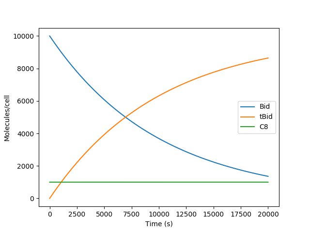
Congratulations! You have created your first model and run a simulation!
Visualization
It is useful to visualize the species and reactions that make a model. We have provided two methods to visualize species and reactions. We recommend using the tools in Kappa and BioNetGen for other visualization tools such as contact maps and stories.
The simplest way to visualize a model is to generate the graph file
using the programs available from the command line. The files are
located in the .../pysb/tools directory. The files to
visualize reactions and species are render_reactions.py and
render_species.py. These python scripts will generate .dot
graph files that can be visualized using several tools such as
OmniGraffle in OS X or GraphViz in all major
platforms. For this tutorial we will use the GraphViz renderer. For
this example we will visualize the mymodel.py file that was
created earlier. Issue the following command, replacing the comments
inside square brackets``[]`` with the correct paths. We will first
generate the .dot from the command line as follows:
[path-to-pysb]/pysb/tools/render_reactions.py [path-to-pysb-model-file]/mymodel.py > mymodel.dot
If your model can be properly visualized you should have gotten no
errors and should now have a file called mymodel.dot. You can
now use this file as an input for any visualization tool as described
above. You can follow the same procedures with the
render_species.py script to visualize the species generated by
your models.
Higher-order rules
For this section we will show the power of working in a programming environment by creating a simple function called “catalyze”. Catalysis happens quite often in models and it is one of the basic functions we have found useful in our model development. Rather than typing many lines such as:
Rule("association",  Enz(b=None) + Sub(b=None, S="i") | Enz(b=1)%Sub(b=1,S="i"), kf, kr)
Rule("dissociation", Enz(b=1)%Sub(b=1,S="i") >> Enz(b=None) + Sub(b=None, S="a"), kc)
multiple times, we find it more powerful, transparent and easy to instantiate/edit a simple, one-line function call such as:
catalyze(Enz, Sub, "S", "i", "a", kf, kr, kc)
We find that the functional form captures what we mean to write: a chemical species (the substrate) undergoes catalytic activation (by the enzyme) with a given set of parameters. We will now describe how a function can be written in PySB to automate the scripting of simple concepts into a programmatic format. Examine the function below:
def catalyze(enz, sub, site, state1, state2, kf, kr, kc):   # (0) function call
    """2-step catalytic process"""                          # (1) reaction name
    r1_name = '%s_assoc_%s' % (enz.name, sub.name)          # (2) name of association reaction for rule
    r2_name = '%s_diss_%s' % (enz.name, sub.name)           # (3) name of dissociation reaction for rule
    E = enz(b=None)                                         # (4) define enzyme state in function
    S = sub({'b': None, site: state1})                      # (5) define substrate state in function
    ES = enz(b=1) % sub({'b': 1, site: state1})             # (6) define state of enzyme:substrate complex
    P = sub({'b': None, site: state2})                      # (7) define state of product
    Rule(r1_name, E + S | ES, kf, kr)                       # (8) rule for enzyme + substrate association (bidirectional)
    Rule(r2_name, ES >> E + P, kc)                          # (9) rule for enzyme:substrate dissociation  (unidirectional)
As shown it takes about ten lines to write the catalyze function (shorter variants are certainly possible with more advanced Python statements).
As shown, Monomers, Parameters, Species, and pretty much
anything related to rules-based modeling are instantiated as objects
in Python. One could write functions to interact with these objects
and they could be instantiated and inherit methods from a class. The
limits to programming biology with PySB are those enforced by the
Python language itself. We can now go ahead and embed this into a
model. Go back to your mymodel.py file and modify it to look
something like this:
# import the pysb module and all its methods and functions
from pysb import *


def catalyze(enz, sub, site, state1, state2, kf, kr, kc):   # function call
    """2-step catalytic process"""                          # reaction name
    r1_name = '%s_assoc_%s' % (enz.name, sub.name)          # name of association reaction for rule
    r2_name = '%s_diss_%s' % (enz.name, sub.name)           # name of dissociation reaction for rule
    E = enz(b=None)                                         # define enzyme state in function
    S = sub({'b': None, site: state1})                      # define substrate state in function
    ES = enz(b=1) % sub({'b': 1, site: state1})             # define state of enzyme:substrate complex
    P = sub({'b': None, site: state2})                      # define state of product
    Rule(r1_name, E + S | ES, kf, kr)                       # rule for enzyme + substrate association (bidirectional)
    Rule(r2_name, ES >> E + P, kc)                          # rule for enzyme:substrate dissociation  (unidirectional)

# instantiate a model
Model()

# declare monomers
Monomer('C8', ['b'])
Monomer('Bid', ['b', 'S'], {'S':['u', 't']})

# input the parameter values
Parameter('kf', 1.0e-07)
Parameter('kr', 1.0e-03)
Parameter('kc', 1.0)

# OLD RULES
# Rule('C8_Bid_bind', C8(b=None) + Bid(b=None, S='u') | C8(b=1) % Bid(b=1, S='u'), *[kf, kr])
# Rule('tBid_from_C8Bid', C8(b=1) % Bid(b=1, S='u') >> C8(b=None) + Bid(b=None, S='t'), kc)
#
# NEW RULES
# Catalysis
catalyze(C8, Bid, 'S', 'u', 't', kf, kr, kc)


# initial conditions
Parameter('C8_0', 1000)
Parameter('Bid_0', 10000)
Initial(C8(b=None), C8_0)
Initial(Bid(b=None, S='u'), Bid_0)

# Observables
Observable('obsC8', C8(b=None))
Observable('obsBid', Bid(b=None, S='u'))
Observable('obstBid', Bid(b=None, S='t'))
With this you should be able to execute your code and generate figures as described in the previous sections.
Using provided macros
For further reference we invite the users to explore the
macros.py file in the .../pysb/ directory. Based on
our experience with modeling signal transduction pathways we have
identified a set of commonly-used constructs that can serve as
building blocks for more complex models. In addition to some
meta-macros useful for instantiating user macros, we provide a set of
macros such as equilibrate. bind, catalyze,
catalyze_one_step, catalyze_one_step_reversible,
synthesize, degrade, assemble_pore_sequential, and
pore_transport. In addition to these basic macros we also provide
the higher-level macros bind_table and catalyze_table which we
have found useful in instantiating the interactions between families
of models.
In what follows we expand our previous model example of Caspase-8
by adding a few more species. The initiator caspase, as was described
earlier, catalytically cleaves Bid to create truncated Bid
(tBid) in this model. This tBid then catalytically activates
Bax and Bak which eventually go on to form pores at the mitochondria
leading to mitochondrial outer-membrane permeabilization (MOMP) and eventual
cell death. To introduce the concept of higher-level macros we will
show how the bind_table macro can be used to show how a family of
inhibitors, namely Bcl-2, Bcl-xL, and Mcl-1 inhibits a
family of proteins, namely Bid, Bax, and Bak.
In your favorite editor, go ahead and create a file (I will refer to
it as ::file::mymodel_fxns). Many rules that dictate the
interactions among species depend on a single binding site. We will
begin by creating our model and declaring a generic binding site. We
will also declare some functions, using the PySB macros and tailor
them to our needs by specifying the binding site to be passed to the
function. The first thing we do is import PySB and then import PySB
macros. Then we declare our generic site and redefine the pysb.macros
for our model as follows:
# import the pysb module and all its methods and functions
from pysb import *
from pysb.macros import *

# some functions to make life easy
site_name = 'b'
def catalyze_b(enz, sub, product, klist):
    """Alias for pysb.macros.catalyze with default binding site 'b'.
    """
    return catalyze(enz, site_name, sub, site_name, product, klist)
def bind_table_b(table):
    """Alias for pysb.macros.bind_table with default binding sites 'bf'.
    """
    return bind_table(table, site_name, site_name)
The first two lines just import the necessary modules from PySB. The
catalyze_b` function, tailored for the model, takes four inputs
but feeds six inputs to the pysb.macros.catalyze function, hence
making the model more clean. Similarly the bind_table_b function
takes only one entry, a list of lists, and feeds the entries needed to
the pysb.macros.bind_table macro. Note that these entries could be
contained in a header file to be hidden from the user at model time.
With this technical work out of the way we can now actually start our
mdoel building. We will declare two sets of rates, the bid_rates
that we will use for all the Bid interactions and the
bcl2_rates which we will use for all the Bcl-2
interactions. These values could be specified individually as desired
but it is common practice in models to use generic values
for the reaction rate parameters of a model and determine these in
detail through some sort of model calibration. We will use these
values for now for illustrative purposes.
The next entries for the rates, the model declaration, and the Monomers follow:
# Bid activation rates
bid_rates = [        1e-7, 1e-3, 1] #

# Bcl2 Inhibition Rates
bcl2_rates = [1.428571e-05, 1e-3] # 1.0e-6/v_mito

# instantiate a model
Model()

# declare monomers
Monomer('C8',    ['b'])
Monomer('Bid',   ['b', 'S'], {'S':['u', 't', 'm']})
Monomer('Bax',   ['b', 'S'], {'S':['i', 'a', 'm']})
Monomer('Bak',   ['b', 'S'], {'S':['i', 'a']})
Monomer('BclxL', ['b', 'S'], {'S':['c', 'm']})
Monomer('Bcl2', ['b'])
Monomer('Mcl1', ['b'])
As shown, the generic rates are declared followed by the declaration
of the monomers. We have the C8 and Bid monomers as we did in
the initial part of the tutorial, the MOMP effectors Bid, Bax,
Bak, and the MOMP inhibitors Bcl-xL, Bcl-2, and
Mcl-1. The Bid, Bax, and BclxL monomers, in addition
to the active and inactive terms also have a 'm' term indicating
that they can be in a membrane, which in this case we indicate as a
state. We will have a translocation to the membrane as part of the
reactions.
We can now begin to write some checmical procedures. The
first procedure is the catalytic activation of Bid by C8. This
is followed by the catalytic activation of Bax and Bak.
# Activate Bid
catalyze_b(C8, Bid(S='u'), Bid(S='t'), [KF, KR, KC])

# Activate Bax/Bak
catalyze_b(Bid(S='m'), Bax(S='i'), Bax(S='m'), bid_rates)
catalyze_b(Bid(S='m'), Bak(S='i'), Bak(S='a'), bid_rates)
As shown, we simply state the species that acts as an enzyme as the
first function argument, the species that acts as the reactant with
the enzyme as the second argument (along with any state
specifications) and finally the product species. The bid_rates
argument is the list of rates that we declared earlier.
You may have noticed a problem with the previous statements. The
Bid species undergoes a transformation from state S='u' to
S='t' but the activation of Bax and Bak happens only when
Bid is in state S='m' to imply that these events only happen
at the membrane. In order to transport Bid from the 't' state
to the 'm' state we need a transport function. We achieve this by
using the equilibrate macro in PySB between these states. In
addition we use this same macro for the transport of the Bax
species and the BclxL species as shown below.
# Bid, Bax, BclxL "transport" to the membrane
equilibrate(Bid(b=None, S='t'),   Bid(b=None, S='m'), [1e-1, 1e-3])
equilibrate(Bax(b=None, S='m'),   Bax(b=None, S='a'), [1e-1, 1e-3])
equilibrate(BclxL(b=None, S='c'), BclxL(b=None, S='m'), [1e-1, 1e-3])
According to published experimental data, the Bcl-2 family of
inhibitors can inhibit the initiator Bid and the effector Bax
and Bak. This family has complex interactions with all these
proteins. Given that we have three inhibitors, and three molecules to
be inhibited, this indicates nine interactions that need to be
specified. This would involve writing nine reversible reactions in a
rules language or at least eighteen reactions for each direction if we
were writing the ODEs. Given that we are simply stating that these
species bind to inhibit interactions, we can take advantage of two
things. In the first case we have already seen that there is a bind
macro specified in PySB. We can further functionalize this into a
higher level macro, namely the bind_table macro, which takes a table
of interactions as an argument and generates the rules based on these
simple interactions. We specify the bind table for the inhibitors (top
row) and the inhibited molecules (left column) as follows.
bind_table_b([[                  Bcl2,  BclxL(S='m'),       Mcl1],
              [Bid(S='m'), bcl2_rates,  bcl2_rates,   bcl2_rates],
              [Bax(S='a'), bcl2_rates,  bcl2_rates,         None],
              [Bak(S='a'),       None,  bcl2_rates,   bcl2_rates]])
As shown the inhibitors interact by giving the rates of interactions or the “None” Python keyword to indicate no interaction. The only thing left to run this simple model is to declare some initial conditions and some observables. We declare the following:
# initial conditions
Parameter('C8_0',    1e4)
Parameter('Bid_0',   1e4)
Parameter('Bax_0',  .8e5)
Parameter('Bak_0',  .2e5)
Parameter('BclxL_0', 1e3)
Parameter('Bcl2_0',  1e3)
Parameter('Mcl1_0',  1e3)

Initial(C8(b=None), C8_0)
Initial(Bid(b=None, S='u'), Bid_0)
Initial(Bax(b=None, S='i'), Bax_0)
Initial(Bak(b=None, S='i'), Bak_0)
Initial(BclxL(b=None, S='c'), BclxL_0)
Initial(Bcl2(b=None), Bcl2_0)
Initial(Mcl1(b=None), Mcl1_0)

# Observables
Observable('obstBid', Bid(b=None, S='m'))
Observable('obsBax', Bax(b=None, S='a'))
Observable('obsBak', Bax(b=None, S='a'))
Observable('obsBaxBclxL', Bax(b=1, S='a')%BclxL(b=1, S='m'))
By now you should have a file with all the components that looks something like this:
# import the pysb module and all its methods and functions
from pysb import *
from pysb.macros import *

# some functions to make life easy
site_name = 'b'
def catalyze_b(enz, sub, product, klist):
    """Alias for pysb.macros.catalyze with default binding site 'b'.
    """
    return catalyze(enz, site_name, sub, site_name, product, klist)

def bind_table_b(table):
    """Alias for pysb.macros.bind_table with default binding sites 'bf'.
    """
    return bind_table(table, site_name, site_name)

# Default forward, reverse, and catalytic rates
KF = 1e-6
KR = 1e-3
KC = 1

# Bid activation rates
bid_rates = [        1e-7, 1e-3, 1] #

# Bcl2 Inhibition Rates
bcl2_rates = [1.428571e-05, 1e-3] # 1.0e-6/v_mito

# instantiate a model
Model()

# declare monomers
Monomer('C8',    ['b'])
Monomer('Bid',   ['b', 'S'], {'S':['u', 't', 'm']})
Monomer('Bax',   ['b', 'S'], {'S':['i', 'a', 'm']})
Monomer('Bak',   ['b', 'S'], {'S':['i', 'a']})
Monomer('BclxL', ['b', 'S'], {'S':['c', 'm']})
Monomer('Bcl2', ['b'])
Monomer('Mcl1', ['b'])

# Activate Bid
catalyze_b(C8, Bid(S='u'), Bid(S='t'), [KF, KR, KC])

# Activate Bax/Bak
catalyze_b(Bid(S='m'), Bax(S='i'), Bax(S='m'), bid_rates)
catalyze_b(Bid(S='m'), Bak(S='i'), Bak(S='a'), bid_rates)

# Bid, Bax, BclxL "transport" to the membrane
equilibrate(Bid(b=None, S='t'),   Bid(b=None, S='m'), [1e-1, 1e-3])
equilibrate(Bax(b=None, S='m'),   Bax(b=None, S='a'), [1e-1, 1e-3])
equilibrate(BclxL(b=None, S='c'), BclxL(b=None, S='m'), [1e-1, 1e-3])


bind_table_b([[                  Bcl2,  BclxL(S='m'),       Mcl1],
              [Bid(S='m'), bcl2_rates,  bcl2_rates,   bcl2_rates],
              [Bax(S='a'), bcl2_rates,  bcl2_rates,         None],
              [Bak(S='a'),       None,  bcl2_rates,   bcl2_rates]])

# initial conditions
Parameter('C8_0',    1e4)
Parameter('Bid_0',   1e4)
Parameter('Bax_0',  .8e5)
Parameter('Bak_0',  .2e5)
Parameter('BclxL_0', 1e3)
Parameter('Bcl2_0',  1e3)
Parameter('Mcl1_0',  1e3)

Initial(C8(b=None), C8_0)
Initial(Bid(b=None, S='u'), Bid_0)
Initial(Bax(b=None, S='i'), Bax_0)
Initial(Bak(b=None, S='i'), Bak_0)
Initial(BclxL(b=None, S='c'), BclxL_0)
Initial(Bcl2(b=None), Bcl2_0)
Initial(Mcl1(b=None), Mcl1_0)

# Observables
Observable('obstBid', Bid(b=None, S='m'))
Observable('obsBax', Bax(b=None, S='a'))
Observable('obsBak', Bax(b=None, S='a'))
Observable('obsBaxBclxL', Bax(b=1, S='a')%BclxL(b=1, S='m'))
With this you should be able to run the simulations and generate figures as described in the basic tutorial sections.
Compartments
We will continue building on your mymodel_fxns.py file and add one
more species and a compartment. In extrinsic apoptosis, once tBid is
activated it translocates to the outer mitochondrial membrane where it
interacts with the protein Bak (residing in the membrane).
Model calibration
One option for model calibration in PySB is PyDREAM, which is an implementation of the DREAM algorithm developed by Vrugt and ter Braak (2008) and Laloy and Vrugt (2012).
Modules
See PySB Modules Reference for further details on the various PySB modules and the options available.
Miscellaneous
Self-export
For anyone who feels a little queasy about self-export, this section will try to explain the rationale behind it.
In order to make model definition feel like a domain-specific language specially designed for model construction, the mechanism for component definition needs to provide three things:
It must provide an internal name so that components can be usefully distinguished when inspected interactively, or translated into various output file formats such as BNGL.
The component object must be assigned to a local variable so that subsequent component declarations can reference it by name using normal Python syntax (including operator overloading).
The object must also be inserted into the data structures of the model object itself.
Without self-export, every component definition would need to manage these points explicitly:
A = Monomer('A')
model.add_component(A)
B = Monomer('B')
model.add_component(B)
This pattern introduces several opportunities for error, for example a name
argument and the corresponding variable name may end up out of sync or the
modeler may forget an add_component call. The redundancy also introduces
visual noise which makes the code harder to read. Furthermore, self-export makes
model modularization much simpler, as components may be defined within functions
without forcing the function to explicitly return them or requiring extra code
in the caller to deal with the returned components.
In addition to Component and its subclasses, the Model constructor also
utilizes self-export, with two differences: The local variable is always named
model, and the name argument is optional and defaults to the full
hierarchical name of the module from which Model() is called, e.g.
pysb.examples.tutorial_a.
Footnotes